Due December 10th, 2021 at 11:59 PM.
In this project, we will use machine learning algorithms to perform image classification. Image classification is the task of predicting the class, or label, of an image out of a set of known images. This is a type of supervised learning, which refers to algorithms that learn a function from labelled datasets.
We will be writing algorithms to do image classification on the MNIST dataset. MNIST consists of tiny 28×28 pixel images of handwritten digits from 0 to 9. A few example images from each are shown below.
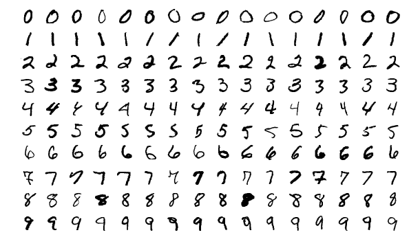
MNIST has 60,000 images to train a classification algorithm, each labelled with the correct digit. In addition, there are 10,000 images which are used for testing the accuracy of the algorithm. We will implement three machine learning algorithms to classify images: nearest neighbors, linear classification, and a neural network.
This project is implemented using the programming language Julia. Before you start, make sure you have followed the Julia install instructions to install Julia locally on your computer. The following topics are covered on this page:
- Getting the Code
- Submitting the Assignment
- Part 0: Intro to Julia
- Project Description
- Task Summary
- Advanced Extensions
Getting the Code
One repository per student will be created for this project.
The invite link to accept the assignment on Github Classroom can be found on Slack.
The code for this assignment runs in Jupyter notebooks on your computer. This command clones the repository:
git clone <ADDRESS>Substitute the address to your repository. Run this command in the folder where you have been keeping your ROB 102 repositories all semester.
Submitting the Assignment
Your submission for this assignment should include your Jupyter notebook, along with the output containing the results and any plots. You may also add new cells to perform further analysis or visualization, as well as Markdown cells to write up your observations and analysis. When you run your cells, the output gets saved in the notebook file. When you push this file to GitHub, you and the instructors will be able to see output such as images, plots, and printed values, on GitHub. You can visualize what your notebook looks like to others on GitHub.
Submitting the code: Tag the verion of the code you wish to submit. See instructions from Project 0.
Modify the LICENSE.txt file to include your name and the year. Make sure the change is committed to your repository.
-
P4 License: In the file
LICENSE.txt, replace<COPYRIGHT HOLDER>with your name. Replace<YEAR>with the current year.
Part 0: Introduction to Julia
This part of the project will not be graded. It is there to help you get used to programming in Julia.
To get familiar with using Jupyter notebooks and programming in Julia, we have created an introductory notebook. The invite link to accept the assignment on Github Classroom can be found on Slack.
Once you have accepted the assignment and created a repository, clone your repository onto your computer, substituting the address to your repo:
git clone <ADDRESS>Launching a Jupyter Notebook
We will use Jupyter notebooks to write code in Julia quickly and easily visualize outputs. To launch a Jupyter notebook which uses Julia, open a Julia interpreter and enter the following commands:
using IJulia
notebook()
A webpage should open on your default browser with the home page for the Jupyter notebook server you just launched. Navigate to the repository you just cloned for Project 4. The page will look something like this:
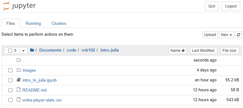
Click on the notebook file, intro_to_julia.ipynb to launch it. To stop the Jupyter notebook server, do Ctrl-C (on Mac, do Cmd-C).
- 4.0: Read through the Intro to Julia Jupyter notebook and complete the exercises.
- Hint: The Julia documentation is a great resource for more details about syntax, built-in functions, and best practices: https://docs.julialang.org/
Project Description
In this project, you will develop three algorithms for image classification on the MNIST dataset:
The invite link to accept the assignment on Github Classroom can be found on Slack.
Part 1: Nearest Neighbors
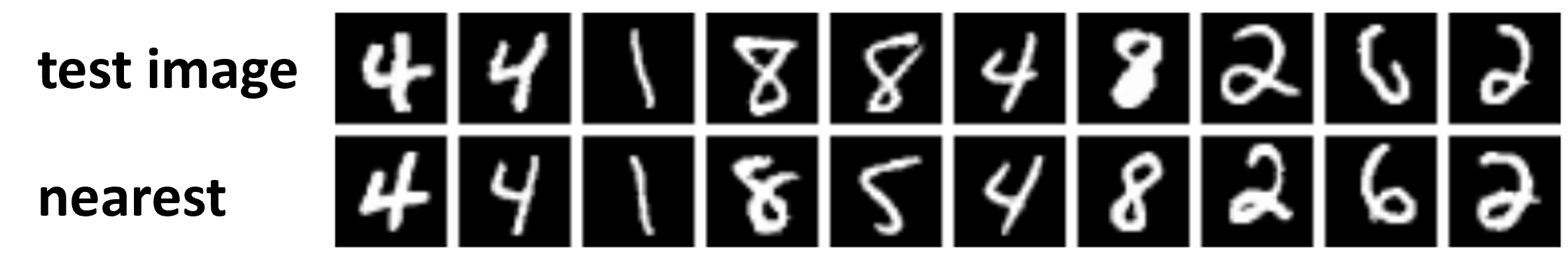
In Part 1 of this project, you will implement a Nearest Neighbor classifier. The nearest neighbor algorithm takes a test image and finds the closest train image, which we call the image's nearest neighbor. Then, it assigns the test image the same label as its nearest neighbor. Here is an example of some MNIST images and their nearest neighbors:
Notebook setup
Open the notebook nearest_neighbors.ipynb by double-clicking it in the web browser. The notebook is made up of cells, which can be text cells (in Markdown) or code cells (in Julia). You can run a cell by selecting the cell and pressing Run.
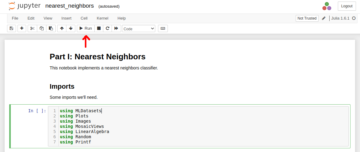
You need to run a cell before you use anything it defines in another cell. For example, you should always run the imports cell when you start the notebook. Similarly, you must run a cell which defines a variable or function before running a cell that uses it. Start by running the import cell at the top of the notebook nearest_neighbors.ipynb to import some dependencies we'll need later on.
The second cell in the notebook loads the MNIST data, provided by the "MLDatasets" Julia library. Run this cell now. The first time you load the data, you'll see a message like this:
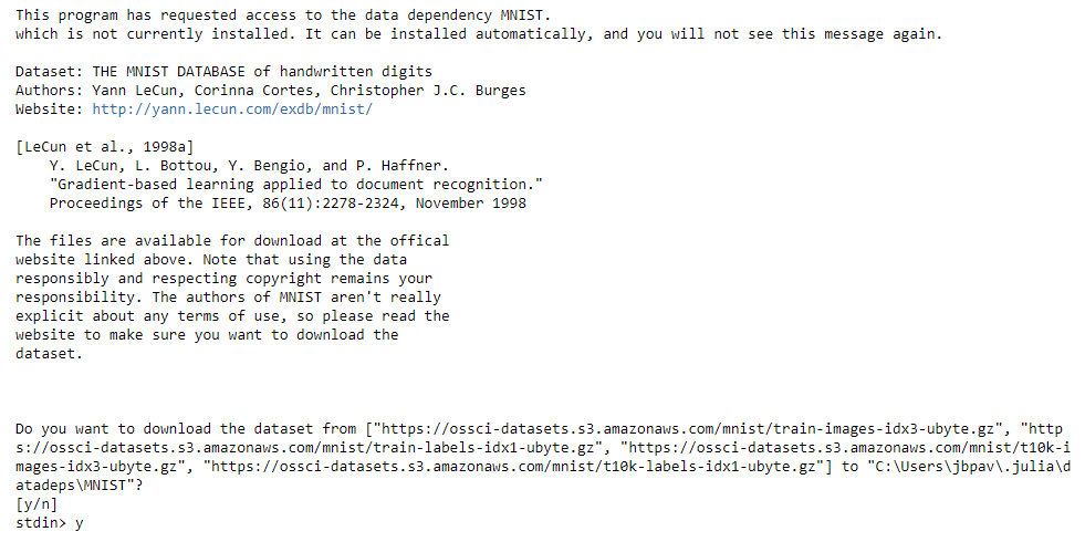
Type y into the box that appears at the top and press enter to download the data in
the default directory. It will take a few minutes for the data to download.
The text in the notebook contains descriptions of how the data is stored and how distance should be calculated. The function compute_distance() in the provided notebook should compute the distance between two image vectors. The function compute_distances() should find the distance between a test image and each of the training images. Use the provided test cells to check that your functions are working correctly.
-
4.1.1: Complete the function
compute_distance()so that it returns the distance between two flattened images. -
4.1.2: Complete the function
compute_distances()so that it returns a vector containing the distance from a test image to each training image.
-
Hint: You should reuse
compute_distance()when implementing thecompute_distances()function.
Finding nearest neighbors
We want to find the nearest neighbor of a test image in the training set. The nearest neighbor of an image is the image with the smallest distance. The function nearest_neighbor() should find the index of the nearest training image to a given test image.
-
4.1.3: Complete the function
nearest_neighbor()so that it returns an integer corresponding to the index of the nearest neighbor to a test image in the training set.
-
Hint: You should reuse
compute_distances()when implementing thenearest_neighbor()function. - Hint: Why do we want the index of the nearest neighbor instead of the image itself? Think of the index as a unique ID for a data point. We can use the index to access the image or its label. We'll see why this is useful later.
We need to classify all N_test images in the test set. The function nearest_neighbors_multi() should return a vector of indices corresponding to the nearest training image for each test image. Again, the notebook contains test cells to help you check that your functions are implemented correctly.
-
4.1.4: Complete the function
nearest_neighbors_multi()so that it returns a vector of integers corresponding to the indices of the nearest neighbor to each test image in the training set.
-
Hint: You should reuse
nearest_neighbor()when implementing thenearest_neighbors_multi()function.
Now, we have the functions we need to implement a Nearest Neighbors image classifier. The function predict_nn_labels() should use the training data x_train and y_train to predict the labels for each test image in x_test.
-
4.1.5: Complete the function
predict_nn_labels()so that it returns a vector of integers corresponding to the class labels for each test image.
-
Hint: You might consider using
nearest_neighbors_multi()when implementing thepredict_nn_labels()function.
Congratulations! You just implemented a machine learning algorithm for image classification. Use the provided cell to check the accuracy of your algorithm. How did you do? What happens to the accuracy when you change the number of training images, N_train? (Remember to rerun the necessary cells when you change the values).
-
4.1.6: Change the value of
N_trainand rerun the prediction step. The value should be between 1 and 50,000. Record your observations.
-
Hint: How do different values of
N_trainaffect the prediction accuracy? The computation time? -
Hint: For very large values of
N_train, you might run out of time (or even memory). Use your reason when deciding which values to try. You will not have time to try them all!
Advanced Extension: k-Nearest Neighbors
In k-nearest neighbors, we try to improve our prediction by finding the \(k\) nearest neighbors to a test image. We perform prediction by letting the neighbors vote on the label for the test image. As an advanced extension, you may complete the k-nearest neighbors algorithm using the template code in the notebook.
- Advanced Extension 4.i: Implement k-nearest neighbors in the provided notebook cells.
- Advanced Extension 4.ii: Experiment with different values of \(k\) and report how \(k\) affects the accuracy. Select a value of \(k\) and compare the accuracy to that of nearest neighbors.
Part 2: Linear Classifiers
Let's see if we can do a bit better at classifying images by learning the parameters for a linear function. This assignment will walk you through implementing a linear classification algorithm for the MNIST dataset. In this section, you will complete the notebook linear_classifier.ipnyb.
The forward pass provides the scores for each class for a given image, using a given set of weights. The forward pass is used at testing time to get the scores used to perform classification. It is also used at training time, to compute the loss for the current best set of weights. In the provided notebook cell, implement the forward pass of a linear classifier.
-
4.2.1: Complete the function
linear_forward()so that it returns the class score for each image.
The backward pass calculates the loss and gradients for a batch of images, given the correct labels for those images and a set of weights. In the notebook, the gradient computation is given. You will implement the support vector machine (SVM) loss computation.
-
4.2.2: Complete the function
svm_loss()to calculate the support vector machine (SVM) loss given the class scores.
-
Hint: You should use
linear_forward()to get the scores needed to compute the loss. - Hint: Don't forget the regularization loss!
Training the classifier
Use the functions you developed to train a linear classifier. Implement a training loop in the provided function which first samples a random batch of images, uses svm_loss() to calculate the loss and gradients, then updates the weight matrix. Loop for the given number of iterations. The number of iterations, learning rate, batch size, and regularization coefficient are given (see the function documentation for details).
-
4.2.3: Complete the function
train_svm()to train the linear classifier.
Testing the classifier
Once you have found a set of weights, you can use them to test your algorithm. Code has been provided to test the accuracy of the network. You need to write the test loop that returns class labels for each test image, using the weights found in training.
-
4.2.4: Complete the function
test_svm()to use the forward pass function to predict a label for each image.
-
Hint: The
linear_forward()function might come in handy again.
You're done! But, you might notice that the learning rate and regularization coefficient have an impact on how good the network does. Try tuning them, and report on how they affect the performance of the classifier and which values work best.
- 4.2.5: Tune the learning rate and the regularization coefficient. See how high you can get your accuracy. Report on your observations.
- Hint: You might consider implementing cross validation to tune these parameters, as discussed in lecture.
Part 3: Neural Network
Our linear classifier can only represent linear functions. A two-layer neural network can represent more complicated functions with a different forward model and a few more learnable parameters. You will implement your own two-layer neural network from scratch in the notebook two_layer_neural_net.ipnyb.
Like in the linear classifier, you will compute the forward pass through the neural network, which calculates the class scores for each image in a batch. In the provided cell, implement the forward pass for a two-layer neural network in the function nn_forward().
-
4.3.1: Complete the function
nn_forward()so that it returns the class scores for each image in the batch, and the hidden layer outputs.
Next, you will compute the SVM loss for the current parameters. This will look very similar to the loss computation in the linear classifier! The gradient computation is provided for you.
-
4.3.2: Complete the function
nn_svm_loss()so that it computes the average SVM loss for the batch of images, and saves it to the variableloss.
-
Hint: Use the
nn_forward()function to get the scores and hidden layer outputs.
Training the network
Now it's time to train the neural network! The function train_nn() should sample a batch of images, call nn_svm_loss() to compute the loss and gradients for the current parameters, then update all the weights and biases using gradient descent.
-
4.3.3: Complete the training loop in the function
train_nn()so that it samples a batch, calculates the loss and gradients, and updates the parameters.
-
Hint: You should update both sets of weights and biases. In the code, these are called
W1,W2,b1, andb2. -
Hint: The weights and biases are stored in
params. Access them usingparams["W1"],params["b1"], etc. Make sure to save the updated parameters back inparams. The gradients are stored similarly. If you save them in a variable calledgrads, you would access them withgrads["W1"],grads["b1"], etc.
Testing the network
Now that your've trained your model, we can test the accuracy of our network. Complete the function test_nn() so that it computes the class scores for a batch of images, then returns the predicted class label for each image.
-
4.3.4: Complete the function
test_nn()to compute the class scores for each image and return the predicted label for the images.
-
Hint: The
nn_forward()function might come in handy again.
Just like in the linear classifier, there are some hyperparameters that you can tune to improve your results. Try changing the learning rate, regularization coefficient, and number of hidden neurons to improve your network's performance.
- 4.3.5: Tune the learning rate, regularization coefficient, and number of hidden neurons. See how high you can get your accuracy. Report on your observations.
- Hint: You might consider implementing cross validation to tune these parameters, as discussed in lecture.
Task Summary
-
P4 License:
In the file
LICENSE.txt, replace<COPYRIGHT HOLDER>with your name. Replace<YEAR>with the current year.
Part 0: Intro to Julia
- 4.0: Read through the Intro to Julia Jupyter notebook and complete the exercises.
Part 1: Nearest Neighbors
-
4.1.1: Complete the function
compute_distance()so that it returns the distance between two images. -
4.1.2: Complete the function
compute_distances()so that it returns a vector of distances between an image and a matrix of training images. -
4.1.3: Complete the function
nearest_neighbor()so that it returns the index of the nearest neighbor to a test image in the training set. -
4.1.4: Complete the function
nearest_neighbors_multi()so that it returns a vector of indices of the nearest neighbors of each test image in the training set. -
4.1.5: Complete the function
predict_nn_labels()to predict labels for a set of test images using nearest neighbors. -
4.1.6: Experiment with the value of
N_trainand record your observations.
Part 2: Linear Classifiers
-
4.2.1: Complete the function
linear_forward()so that it returns the class score for each image. -
4.2.2: Complete the function
svm_loss()to calculate the SVM loss given the class scores. -
4.2.3: Complete the function
train_svm()to train the linear classifier. -
4.2.4: Complete the function
test_svm()to use the forward pass function to predict a label for each image. - 4.2.5: Tune the learning rate and the regularization coefficient and report your observations.
Part 3: Neural Network
-
4.3.1: Complete the function
nn_forward()so that it returns the class score and hidden layer outputs for each image. -
4.3.2: Complete the function
nn_svm_loss()to calculate the SVM loss given the class scores. -
4.3.3: Complete the function
train_nn()to train the neural network. -
4.3.4: Complete the function
test_nn()to use the forward pass function to predict a label for each image. - 4.3.5: Tune the learning rate, regularization coefficient, and number of hidden neurons, and report your observations.
Advanced Extensions
- Advanced Extension 4.i: Implement the k-nearest neighbors algorithm.
- Advanced Extension 4.ii: Experiment with different values of \(k\).