Due November 1st, 2021 at 11:59 PM.
In Project 1, we saw that we can control the robot to maintain a goal distance to the wall by correcting the control signals based on the observed sensor data. Now, we want the robot to be able to autonomously navigate to a goal location.
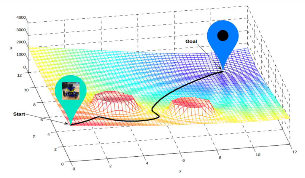 In Project 2, we will accomplish autonomous navigation using potential field control. We can imagine that our goal is a magnet, pulling the robot towards it. We can treat obstacles like repelling forces, pushing the robot away. If we combine these two forces, we might get a potential field that looks like the example on the left. To get to the goal, our robot can follow the path of least resistance, moving in the direction of the strongest force at its location at each time step.
For this project, you will write code in C++ to calculate the potential fields the robot needs to reach a goal without colliding with any obstacles. You will be given a map which tells you where the obstacles are, along with a start and goal position.
This project will be done in teams of 2 or 3. The instructors will assign teammates.
- Getting the Code
- Submitting the Assignment
- Code Overview
- Project Description
- Task Summary
- Advanced Extensions
Getting the Code
One repository per team will be created for this project. All teammates will have access to the repository and will be able to view it and make changes. All teammates will share ownership of the code and receive credit for writing the code through the license file.
The invite link to accept the assignment on Github Classroom can be found on Slack.
Create a GitHub Classroom team named P2 UM Team # for UM students, and P2 Berea Team # for Berea students. Replace # with the team number assigned to you. See Project 1 instructions for more details.
Some parts of the provided code run on your comupter, in a Docker container. Others run on the robot. You will be cloning the repository on both your computer and the robot. This command clones the repository:
git clone <ADDRESS>Substitute the address to your repository. On the robot, run this command in the home directory of the Raspberry Pi, in a terminal opened in a VSCode remote session to the robot (see the robot tutorial). Use the SSH address to clone the repository on the robot (see instructions here).
On your computer, run the clone command in the folder you created for ROB 102 code in Project 0. For most of you, that is a folder called "rob102-code", or something similar, in your Documents folder. Use cd in your terminal to go to this folder before running the clone command.
Submitting the Assignment
Your submission for this assignment should include your code and a project webpage. You should make one submission for your team. Teammates will be graded together.
Modify the LICENSE.txt file to include the names of all teammates. Make sure the change is committed to your repository.
-
P2 License: In the file
LICENSE.txt, replace<COPYRIGHT HOLDER>with the names of all teammates, separated by commas. Replace<YEAR>with the current year.
Submitting the code: Tag the verion of the code you wish to submit. See instructions from Project 0.
Submitting the web page: Create a web page for your implementation of the potential field navigation algorithm. You can use Google Sites, create a project page on a GitHub repository, or use your favorite method to create a website. Note that if you chose to use GitHub pages, you will need to create a separate, public repository. Include at least one video demo as well as a brief summary and discussion of your algorithm. Details about what to include can be found at the end of the project description. Include the link to your project page in the README.md file.
-
P2 Webpage:
Create a web page for your implementation of the potential field navigation algorithm. Include the link to your project page in the
README.mdfile. Include at least one video demo as well as a brief summary and discussion of your algorithm.
Grading Breakdown
This project will be graded as follows:
- Attractive Field Navigation Live Demo (in-class): (2 points) Part 1 of the project will be demonstrated on the robot, in class on October 27th.
- Potential Field Navigation Live Demo (in-class): (2 points) Part 3 of the project will be demonstrated on the robot, in class on November 3rd. You can use whichever implementation of the distance transform and potential field you choose.
- Attractive Field Navigation Video Demo: (2 points) On your website, include at least one video of your robot navigating with an attractive field, as described in Part 1. For full credit, include multiple examples of start and goal locations, and maps.
- Distance Transform Photo Demo: (3 points) On your website, include photos of all implementations of your distance transform, as described in Part 2 (you can take screenshots of the web app). For full credit, include multiple examples of maps.
- Potential Field Navigation Video Demonstration: (3 points) On your website, include at least one video of your robot navigating with a potential field, as described in Part 3. You can use whichever implementation of the distance transform and potential field you choose. Please make the method you used to create the video clear on your website. For full credit, include multiple examples of start and goal locations, and maps. You might also consider including examples of failure cases.
- Discussion: (3 points) On your website, include a brief discussion and analysis of your design choices (see reflection questions).
Code Overview
There are three different code executables that can be run for Project 2:
-
Navigation web server:
This code is stored in
src/web_server.cppand runs in the Docker container, running on your laptop. -
Robot potential field navigation:
This code is stored in
src/robot_potential_field.cppand runs on the robot. -
Tests:
There is one test for Project 2, for Part 0, that is written in
src/tests/test_graph.cppand runs in the Docker container, running on your laptop.
Running the Webapp in the Docker
Follow the instructions in the Webapp Tutorial. There is also a video demonstration linked on Slack.
Running Potential Field Navigation on the Robot
The code to perform potential field navigation on the robot is in src/robot_potential_field.cpp. Before you run the code, you should make a map of the environment you want to run in. Then, run the localization using the map you just made (see Lab 5).
To compile and run potential field navigation on the robot, connect to the robot using VSCode (as described in the robot tutorial). Then, from inside the repository you cloned onto the robot for Project 2, compile as follows:
cd build
cmake -DOMNIBOT=On ..
make
Do not forget the argument -DOMNIBOT=On when running CMake. This is how the compiler knows whether to compile the robot code (which is not compiled by default in the Docker). To run the potential field controller, in the build folder where you compiled, do:
./robot_potential_field [PATH/TO/MAP] [goal_x] [goal_y]The map is stored in ~/botlab-bin/maps/current.map. Use that path if you did not move the map since creating it. You can also pass in goal_x and goal_y, the global position of the goal, relative to the starting position of your map, in meters. If you do not pass these in, they will default to zero.
When you pass in arguments to the code, do not include the square brackets.
Provided Utility Functions
To use provided functions, all you need to do is include the correct header file. The needed header files should already be included in the templates. Check the header files (in folder include/autonomous_navigation/) for all the functions available, and the associated documentation. Some robot functions, including drive(vx, vy, wz), and some other helpers, are the same as in Project 1. Below are a few of the functions you will likely find helpful, from the header include/autonomous_navigation/utils/graph_utils.h (implemented in src/utils/graph_utils.cpp). Other than those marked, these are implemented for you.
-
int cellToIdx(int i, int j, const GridGraph& graph): (TODO, see Part 0) Given a cell rowiand columnjin the graph, calculates the index where the data for the cell is stored. -
Cell idxToCell(int idx, const GridGraph& graph): (TODO, see Part 0) Given an index, calculates the corresponding cell rowiand columnjin the graph. -
bool loadFromFile(const std::string& file_path, GridGraph& graph): Loads graph data from a file. Calls theinitGraph()function. -
void initGraph(GridGraph& graph): Initializes the graph data. Notably, sets the distance transform to all zeros. -
bool isLoaded(const GridGraph& graph): Returns true if the graph has been loaded and false otherwise. -
Cell posToCell(float x, float y, const GridGraph& graph): Given a global positionxandy, in meters, calculates the corresponding cell in the graph. -
std::vector: Given a cell in the graph, calculates the corresponding global position in meters.cellToPos(int i, int j, const GridGraph& graph) -
bool isCellInBounds(int i, int j, const GridGraph& graph): Checks whether a given cell is in the bounds of the graph. -
bool isIdxOccupied(int idx, const GridGraph& graph): Checks whether a given index is occupied. -
bool isCellOccupied(int i, int j, const GridGraph& graph): Checks whether a given cell is occupied. Warning: This only works ifcellToIdx()is implemented. -
std::vector: Returns a list of the indices of the neighbors of the cell at a given index in the graph. Warning: This only works iffindNeighbors(int idx, const GridGraph& graph) cellToIdx()andidxToCell()are implemented.
The following structs are provided:
-
Cell: For representing a cell in the graph.
wherestruct Cell { float i, j; };iis the row of the cell, andjis the columns of the cell. -
GridGraph: For storing map data.
The member variablesstruct GridGraph { GridGraph() : width(-1), height(-1), origin_x(0), origin_y(0), meters_per_cell(0), collision_radius(0.15), threshold(-100) { }; int width, height; // Width and height of the map in cells. float origin_x, origin_y; // The (x, y) coordinate corresponding to cell (0, 0) in meters. float meters_per_cell; // Width of a cell in meters. float collision_radius; // The radius to use to check collisions. int8_t threshold; // Threshold to check if a cell is occupied or not. std::vector<int8_t> cell_odds; // The odds that a cell is occupied. std::vector<float> obstacle_distances; // The distance from each cell to the nearest obstacle. };widthandheightstore the graph width and height, in cells. The variablesorigin_xandorigin_ycorrespond to the global position in meters of the cell(0, 0). This allows us to determine where the origin of the map is. The variablemeters_per_cellcontains the size of each cell, in meters. Finally, thecell_oddsvariable is a vector containing the odds value of each cell. The odds value and organization of the graph was covered in Lab 4.
Project Description
This assignment has the following parts:
- Part 0: Indexing into the Grid Graph
- Part 1: Creating an attractive goal potential field
- Part 2: Implementing the Distance Transform algorithm
- Part 3: Creating a potential field and performing navigation
We also provide an advanced extension to implement the distance transform with Euclidean distance, as discussed in lecture. Most of your time should be spent on Parts 2 and 3.
We will be compiling and executing all the code written on your computer in a Docker container. We have created a web app which you can use to visualize your code. Review the webapp tutorial and make sure that you can run the webapp in the Docker container before continuing with this assignment.
Part 0: Grid Graph
Information about the map for a particular environment is stored in a provided struct called GridGraph, described in the code overview. You can visualize the available maps using the web app.
You should complete the functions cellToIdx() and idxToCell(), which convert between cells and indices as discussed in Lab 4. You can use these functions for the following parts of the project.
-
P2.0.1: In the file
graph_utils.cpp, complete functionscellToIdx()andidxToCell().cellToIdx()should accept a cell coordinate and a graph as arguments, and return anintcontaining the corresponding array index for the cell.idxToCell()should accept an array index and a graph as arguments, and return aCellcontaining the corresponding cell coordinate for the array index.
We have provided a test script to check your indexing functions. Compile your code in the Docker container (using the instructions in the tutorial), then run the test script in the Docker like this:
cd /code/build
cmake ..
make
./test_graph
The tests should pass before you move on to the next step. You may add more tests if you would like.
Part 1: The Goal Field
In this part, you will write an attractive field to pull the robot towards the goal location. You will test your function on the robot. You can also use the web app to test the function.
First, complete function createAttractiveField() in file src/potential_field/potential_field.cpp so that it accepts the current graph and a goal cell and returns a vector representing the attractive field. The field should be a vector with the same length as the graph cell data, and should be indexed the same way.
Next, modify the code in src/robot_potential_field.cpp so that it uses the function createAttractiveField() to drive to a goal. Create a map using the localization code provided, and pick a goal in that map. The template code uses the provided function localSearch() to get a 2D vector pointing towards the next location in the potential field to explore. Use this vector to create velocity commands to send to the robot. At this point, your robot will not be able to avoid obstacles, so make sure you pick a start and goal position so that your robot doesn't collide with anything.
-
P2.1.1: In the file
potential_field.cpp, complete functioncreateAttractiveField()to return a vector corresponding to an attractive potential field towards a given goal. -
P2.1.2: Modify
robot_potential_field.cppso that it gets an attractive potential field to a goal, then drives in the direction returned by thelocalSearch()function. When the robot reaches a minimum in the field,localSearch()will return a vector of zeros. Test your code on the robot.
- Hint: An attractive field where the value of each cell is the distance to the goal location works when this is the only field.
- Hint: Use your indexing functions to convert between Cell types and indices, and your distance function to calculate distances between cells.
- Hint:
You can visualize your attractive field in the web app by setting the vector
potential_fieldin the functioncreatePotentialField()to be equal to the attractive field. The field will be visualized when you plan using the "Potential Field" option in the web app. - Hint:
The local search function returns a vector containing three elements:
{vx, vy, grad}. The first two,vxandvy, make a unit vector (with magnitude 1) pointing in the direction of the largest decrease in potential from the current location of the robot. The last element represents the magnitude of decrease in potential between the cell the robot is in, and the next cell in the direction of the vector. You might want to use it to control the velocity of the robot in your navigation algorithm.
Part 2: Distance Transform
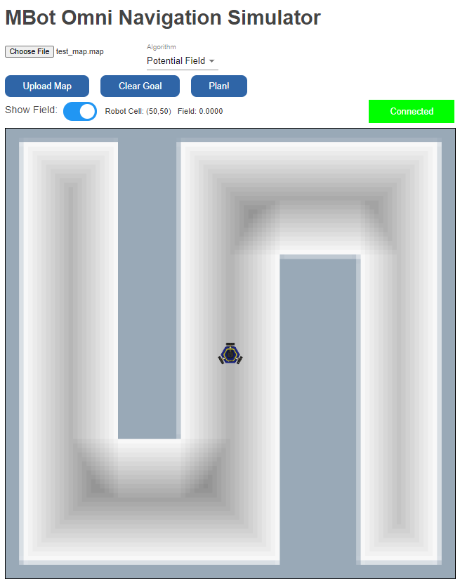
In this part, you will implement a distance transform, which will calculate the distance from each cell to the nearest obstacle. This part can be implemented entirely on your computer in the Docker, using the web app (no robot needed). It should look something like the image below. The grey cells represent smaller distances to the nearest obstacle, and the white cells represent higher distances.
We will be implementing a binary distance transform, which calculates the distance from each cell to the nearest occupied cell. For occupied cells, the distance should be zero.
We will start by implementing a slow version of the distance transform which gives us the Euclidean distance to each cell. Implement this algorithm in the function distanceTransformSlow() located in src/potential_field/distance_transform.cpp. For each unoccupied cell, calculate the distance between the current cell and every occupied cell in the graph. Store the smallest distance in the graph.obstacle_distances vector.
-
P2.2.1:
In the
distance_transform.cppfile, complete functiondistanceTransformSlow(). It should accept a graph and populate thegraph.obstacle_distancesvector with the Euclidean distance to the nearest occupied cell.
You should make sure to test your algorithm on multiple different maps. You can use the web app to visualize the distances as a gradient. It should look like the image at the beginning of this page.
- Hint: You can visualize your transform in the web app by modifying the function
distanceTransform()so that it callsdistanceTransformSlow(). You should be able to see the distance transform when you toggle "Show Field" in the web app, after uploading the map file. - Hint: Can you make your algorithm any faster?
Next, we will implement a much faster algorithm for computing the distance transform, but which computes the Manhattan distance from each unoccupied cell to the nearest occupied cell. Implement this algorithm in the function distanceTransformManhattan() located in src/potential_field/distance_transform.cpp. You should implement the 2D Manhattan distance transform algorithm presented in lecture. You can visualize your distance transform by modifying the function distanceTransform() so that it calls distanceTransformManhattan(), just like for the slow version you completed.
-
P2.2.2:
In the
distance_transform.cppfile, complete functiondistanceTransformManhattan(). It should accept a graph and populate thegraph.obstacle_distancesvector with the Manhattan distance to the nearest occupied cell, using the 2D Manhattan distance transform algorithm presented in lecture.
Part 3: Potential Field Navigation
Now, you will combine the attractive field from Part 1 and the distance transform from Part 2 into a single potential field. Transform the distance transform stored in graph.obstacle_distances into a repulsive field in function createRepulsiveField() in file src/potential_field/potential_field.cpp. Then, modify createPotentialField() in the same file to combine the two. You might want to modify createAttractiveField() for this part.
You should test your field in the web app, and when you are satisfied with the result, try it out on the robot. Modify the code in src/robot_potential_field.cpp to call the function createPotentialField(). The robot should now be able to navigate without colliding into obstacles. It will only avoid obstacles that are in its map, not dynamic obstacles, like people walking in front of it, so be careful!
-
P2.3.1:
In the
potential_field.cppfile, complete functioncreateRepulsiveField(). It should create a repulsive field based on the distance transform ingraph.obstacle_distances. -
P2.3.2:
In the
potential_field.cppfile, complete functioncreatePotentialField(). It should combine the attractive and repulsive fields into a single potential field which can be used to navigate to a goal. -
P2.3.3:
Modify the
robot_potential_field.cppfile to use functioncreatePotentialField()to get a potential field for a given map and goal, and navigate the robot using the field.
- Hint: The distance transform is HIGH in places that are far from an obstacle and LOW in places that are close to an obstacle. This is the opposite of the repulsive field, which should have HIGH potential near an obstacle and LOW potential far from an obstacle. What kind of function can you apply to the distances to convert the distance transform to a field?
- Hint: Experiment with a few different functions and parameters to find one that works. You should make sure that the function works for a variety of start and goal locations and maps.
Project Webpage: Results & Reflection Questions
On your project webpage, include a brief description (a few sentences) of your approach for each part. Include lots of images of how your algorithm works on the web app and the robot, as well as at least one video demo of your robot completing potential field navigation in Part 3. You might also consider taking videos of tests you complete on the web app using a screen recording software.
Include a discussion section on the web page, where you discuss the following:
- The strengths of your potential field navigation algorithm
- The limitations of your potential field navigation algorithm
- How you might improve the algorithm (include at least one idea)
In addition, consider these questions:
- Can you make the naive distance transform any faster (without implementing the fast algorithm we discussed in lecture)? If so, consider trying your idea!
- How does the Euclidean distance transform differ from the Manhattan one? How do they compare in terms of speed?
- What function did you select for your attrative and repulsive fields? How did you combine them to create a potential field?
- When and why does your potential field algorithm fail?
Include images or videos whenever possible to illustrate your points. Keep the discussion brief: it should be no longer than two or three paragraphs.
Advanced Extension: Euclidean Distance Transform
Notes on the algorithm: Fast Euclidean Distance Transform. The notes describe an algorithm presented in a research paper which is available here.
As an advanced extension, you can implement the fast Euclidean distance transform described in the notes linked above. The function distanceTransformEuclidean2D() is provided in the file src/potential_field/distance_transform.cpp to implement the algorithm. You may use function distanceTransformEuclidean1D() to implement the 1D version of the algorithm which is used within the 2D algorithm.
-
Advanced Extension P2.2.i (2 extension points):
In the
distance_transform.cppfile, complete functiondistanceTransformEuclidean2D()so that it uses the fast Euclidean distance transform algorithm from lecture, and stores the result ingraph.obstacle_distances.
Task Summary
-
P2 License:
In the file
LICENSE.txt, replace<COPYRIGHT HOLDER>with the names of all teammates, separated by commas. Replace<YEAR>with the current year. -
P2 Webpage:
Create a web page for your implementation of the potential field navigation algorithm. Include the link to your project page in the
README.mdfile. Include at least one video demo as well as a brief summary and discussion of your algorithm. -
P2.0.1:
In the file
graph_utils.cpp, complete functionscellToIdx()andidxToCell(). -
P2.1.1:
In the file
potential_field.cpp, complete functioncreateAttractiveField()to return a vector corresponding to an attractive potential field towards a given goal. -
P2.1.2:
Modify
robot_potential_field.cppso that it gets an attractive potential field to a goal, then drives in the direction returned by thelocalSearch()function. When the robot reaches a minimum in the field,localSearch()will return a vector of zeros. Test your code on the robot. -
P2.2.1:
In the
distance_transform.cppfile, complete functiondistanceTransformSlow(). It should accept a graph and populate thegraph.obstacle_distancesvector with the Euclidean distance to the nearest occupied cell. -
P2.2.2:
In the
distance_transform.cppfile, complete functiondistanceTransformManhattan(). It should accept a graph and populate thegraph.obstacle_distancesvector with the Manhattan distance to the nearest occupied cell, using the 2D Manhattan distance transform algorithm presented in lecture. -
P2.3.1:
In the
potential_field.cppfile, complete functioncreateRepulsiveField(). It should create a repulsive field based on the distance transform ingraph.obstacle_distances. -
P2.3.2:
In the
potential_field.cppfile, complete functioncreatePotentialField(). It should combine the attractive and repulsive fields into a single potential field which can be used to navigate to a goal. -
P2.3.3:
Modify the
robot_potential_field.cppfile to use functioncreatePotentialField()to get a potential field for a given map and goal, and navigate the robot using the field.
Advanced Extensions
-
Advanced Extension P2.2.i (2 extension points):
In the
distance_transform.cppfile, complete functiondistanceTransformEuclidean2D()so that it uses the fast Euclidean distance transform algorithm from lecture, and stores the result ingraph.obstacle_distances.